Radio Monitoring

Frequency-Scan based Direction Finding

Using a magnetic loop antenna makes it possible to determine the direction of a received signal. So transmitters can be located by direction. The goal is, to do this for all transmitters in a frequency band at once.

For better reliability, at least three frequency-scans should be performed successively with the loop oriented north-south (NS) and another three scans with the loop oriented east-west (EW). This can be done with the program AR5000RA, choosing the feature “Monitor” > “Observe frequency band”. The mean of the measured agc-data of each series gives the spectral signals S(NS) and S(EW). So for each frequency there exists now a pair of signals.

At my receiving-site at Algermissen, northern Germany (52° 15’ 9’’ N 9° 58’ 43’’ E) I recorded the agc between 10 and 300 kHz with a resolution of 2 kHz as described above. I chose daytime for scanning because signals exhibit less variance than during nighttime. I used a vertical mounted loop antenna as described in the setup. The resulting rf-spectrum is shown here:

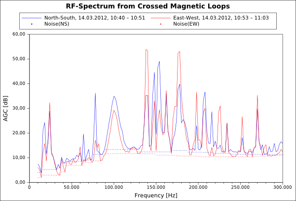
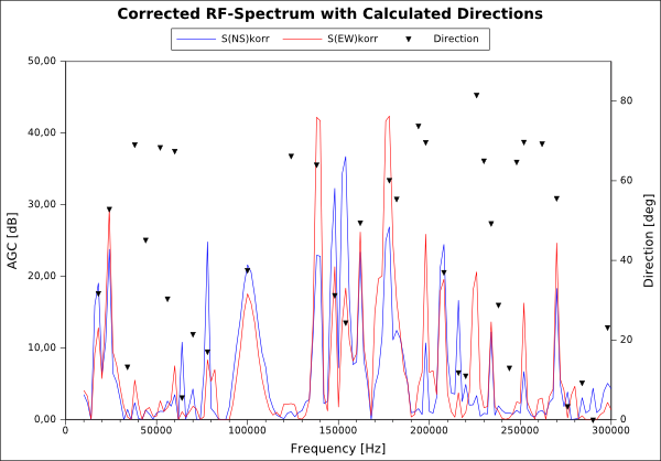
The signals S(NS) and S(EW) are biased by different amounts of noise, which first must be subtracted from the spectrum. The spectrum of noise can be determined by a simple procedure: Within an interval of 20 adjacent frequencies the sample with the lowest agc-level is taken as representative. This procedure is subsequently performed over all frequencies of the north-south and the east-west scan respectively. The resulting curves of spectral noise-floor are plotted as dotted lines in the above graph. After subtraction of the noise the corrected rf-spectrum is shown here:

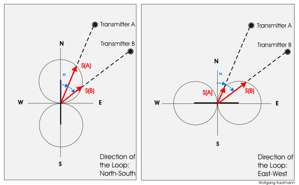
Now we can start to calculate the angle alpha from north to the line connecting the receiving-site with the transmitter-site. The following diagram shows two transmitter-sites A, B and their signal paths towards a vertical mounted loop antenna oriented north-east and east-west respectively. The horizontal spatial variation of the antenna’s sensitivity is represented by two circles surrounding the antenna. The length of the red arrows S(A) and S(B) represent the signal strength produced by the antenna at each orientation for the both transmitter-sites. As can be seen each transmitter-site produces a unique signal difference: S(A, NS) - S(A, EW) for transmitter A and S(B, NS) - S(B, EW) for transmitter B:

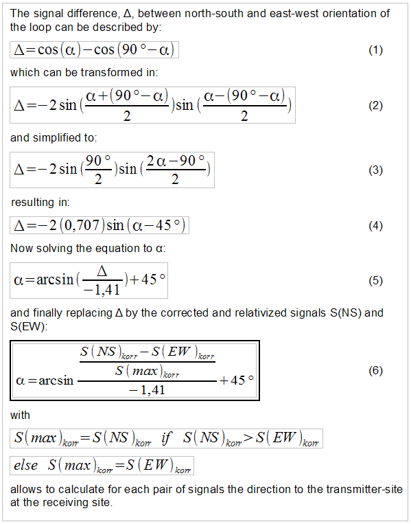
Using equation (6) the directions are calculated for all signals of the above frequency scan: see the marks in the graph of the corrected rf-spectrum. Because of the symmetry of the horizontal spatial responsivity of the loop antenna the calculated alpha must be extended to four directions: alpha / 180° - alpha / 180° + alpha / 360° - alpha. To get an idea, how well this method works a short comparison has been performed:

Frequency	Transmitter	Direction	Calculated Directions
24 kHz	DHO38	300°	53°	127°	233°	307°
60 kHz	MSF	294°	67°	113°	247°	293°
78 kHz	DCF77	195°	17°	163°	197°	343°
148 kHz	DDH47	356°	31°	149°	211°	329°
198 kHz	BBC Droitwich	275°	70°	110°	250°	290°
216 kHz	RMC Romoules	199°	12°	168°	192°	348°
226 kHz	PR Solec Kujawsky	78°	81°	99°	261°	279°