
Radio Meteor Reflection Geometry
First Steps
Here I will present some results of joint radio meteor observations of Mike German, Hayfield, UK and me (Wolfgang Kaufmann, Algermissen, Germany) using GRAVES-Radar as a distant transmitter. The Graves Radar is located at 47° 20' 52" N, 5° 30' 59" W near Dijon, France. It is a space surveillance system to primarily determine the Keplerian elements of the orbits of satellites. It transmits a constant carrier at 143.050 MHz with very high power. The radar beam sweeps over the southern sky from 90° east to 270° west with a constant vertical elevation angle from 15° to 40°. The ionized meteor trails are produced mostly within a height of 80 – 110 km above sea level. At the height of 100 km the sweeping radar beam produces a banana shaped footprint with a width of about 250 km (see fig. 1). Because of sidelobes the sky north of the transmitter must be suspected to be illuminated selectivly also. However the radiation of the sidelobes is much less powerful than that of the main beam. Navaro et al. did some skymapping by systematic analysing radar-reflections by the overflying International Space Station. From their findings the footprint of at least two major sidelobes in the northern vicinity of the transmitter site can be derived (see fig. 1). Also in fig. 1 you will find plotted the receiver locations of Mike and me. Whereas from Algermissen the complete footprint can be observed the situation at Hayfield is different due to nearby hills. A simulation with the software Radio Mobile v. 11.4.8 indicates that beyond a distance of about 1000 km the signal strength will decline rapidly there. So at Hayfield the southeast part of the footprint will not contribute much to the reception of radio meteors.
Fig. 1: Approximate footprint of the GRAVES-Radar beam at a height of 100 km above sea level (coordinate reference system WGS84). The localisation of sidelobes is a rough estimation derived from Navaro et al. (see text). The relevant field of view from each receiver site is indicated over a distance of 1000 km.

We employed varying receiving equipment: an AOR AR5000, an ICOM PCR1000 and a FUNcube Dongle Pro+. All of them produce reliable results. Discone antennas (at Mikes site with a preamplifier) were utilised. In USB mode the received pings from meteor reflections were fed to a computer's soundcard and registered by the software HROFFT 1.0.0f.
Comparing our radio observations of the Leonids 2014 almost no coincidence of the meteor pings received at our sites can be detected (examples see fig. 2). It must be assumed that we received reflections from different meteors.
Fig. 2: Overlay of horizontal waterfall diagrams generated by HROFFT during shower peak of the Leonids. The identified meteor pings were indicated by vertical lines at the bottom of the diagram, the field above graphically represents the ping in the frequency domain. Yellow: Hayfield, green: Algermissen.

Furthermore a comparison of our overdense meteor events with vhf dx-clusters of radio amateurs results in the discovery of additional long-lasting meteor echoes, neither of us has received. Obviously the reception of reflected radio waves from meteor trails displays a high spatial dependency. Fig. 3 gives a basic idea of the spatial distribution of reflected radar waves. More about reflection geometry you will find in this paper from DJ5HG (German language).
Fig. 3: GRAVES radar waves are reflected at an ionized meteor trail resulting in an illuminated belt. Its projection on the surface of the earth results in small zone of radio reception. The graph shows the easier to construct situation of perpendicular incidence of radar waves on the meteor trail.

So a common observation of an identical meteor trail via reflected radio waves would be a rare event for separate locations; it would be possible only for stations lying within the small stripe of reflected radar waves. The position of the stripe on the surface of the earth depends on the angle of incidence of the meteor trail within the footprint of GRAVES radar beam.
From this finding the question arises whether this spatial dependency has an influence on the overall count of radio meteors. To answer this we observed the Geminids 2014 during a time span centered to its predicted shower peak. Fig. 4 shows the result of our measurements. The registered counts/h at the two receiving locations are normalised to their corresponding means i.e. 44.7 counts/h at Algermissen and 30.2 counts/h at Hayfield respectively for the chosen time span. The lower counts at Hayfield are probably due to the reduced observable footprint (see Fig. 1).
Fig. 4: Three days of radio observation of the Geminids centered to the predicted shower peak at Dec. 14th.
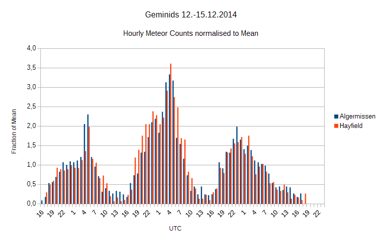
As can be seen from fig. 4 the normalised course of the counts is very consistent; at Dec. 14th 4:00 h UTC a total shower maximum could be verified by both measurements. Also local maxima can be detected from both measurements at Dec. 13th 5:00 h and 23:00 h UTC.
Concluding it becomes evident that each radio observer registers only a fraction of all incident meteors within the footprint of GRAVES radar beam. Yet the course of these recordings is consistent.
Quantification of Coincidence
In a further approach to the question of receiving identical meteors at different locations we carried out a quantitative investigation. For this purpose we employed more directive antennas to observe a common space. At Algermissen a HB9CV antenna and at Hayfield a 2 element 144MHz LFA-Q Super-Gainer Quad Style Yagi were utilised. Each antenna was provided with a preamp. As receiver an ICOM PCR1000 at Hayfield and a FUNcube Dongle Pro+ at Algermissen were used. We applied Spectrum Lab (SL) as new logging software. A new conditional action script for logging of meteors was written based on Simon Dawes' work. In addition to automatically saved spectrograms it writes a csv-file with all relevant data of a detected meteor signal. You can download the script (.txt) and the SL-environment (.usr) here. The script also tests every registered signal for its frequency shift as a valuable criterion to identify interference and writes the result in the csv-file (TestC). Mike performed a thorough analysis of the mainly occuring types of interference and the benefits and shortfalls of the TestC-algorithm. Read more on his findings here. Our testing of the script shows that signals with a TestC-value > 8 dB could be identified as interference in almost all cases. These signals were excluded from further processing. Synchronised timing of the computers was achieved by internet time servers.
We choose a 72 h time-period during the draconids (16:00 UT, 07.10.2015 to 15:59 UT, 10.10.2015). We registered 3702 and 2004 meteor signals at Algermissen and Hayfield respectively. Time resolution of the logging is 1 s. Looking for time differences <= 1 s between both data-sets reveals 103 coincident meteor signals. To answer the question whether this coincident events are only random a Monte Carlo simulation was used. The following model was adopted: Two pots, one for Hayfield, pot(H), and one for Algermissen, pot(A), contain each 259200 balls (=seconds of observations). Pot(H) holds 2004 black (=pings) and 257196 white balls, pot(A) holds 3702 black (=pings) and 255498 white balls. Concurrently from each pot one ball is taken by random and put away. This is repeated until the pots are empty. Thereby each concurrent drawing of two black balls is counted. The complete procedure is repeated 10.000 times. It delivers a distribution of random coincident events shown in fig. 5.
Fig. 5: Resulting distribution from the Monte Carlo simulation described in text.

The mean of this distribution is 28.7 random coincident events.
With a probability of 99.9 % more than 46 coincident events are no more a
result of randomness. So indeed there exists a small fraction of meteors
that reflect GRAVES-radar beam in a way it can be received from both
locations.
Analysis of Spectrograms of GRAVES Radar-Wave Reflections by Meteors
For a fine structure analysis of meteor reflections the following hardware has been employed: a HB9CV antenna directed towards GRAVES transmitter, low noise amplifier (LNA 4000, HF-Berg) and a FUNcube Dongle Pro+ (FCD+). The FCD+ Frequency Control Program was used to set the FCD+ to 143.049 MHz. At this frequency my FCD+ exhibits an offset of about +110 Hz, so the unbiased radar signal would appear at 1110 Hz in the baseband (provided that GRAVES transmitter frequency is 143.050.000 Hz). Everything else is done with Spectrum Lab (SL). To detect and record the reflected radar waves with SL I built a script (.txt) based on Simon Dawes' work and an appropriate environment (.usr). You can download it here. The recorded .wav-files were analysed with SL subsequently. Recordings were done from 21th of July to 2nd of August 2015 at Algermissen, Germany.
The analysis of the spectrograms reveals a lot of unique signal signatures. To catalogue the distinguishable echoes I start with the description of a spectrogram of a complete meteor signal (Rendtel, J. and R. Arlt (eds.): Handbook for Meteor Observers. Potsdam IMO, 2015), consisting of a head echo and a trail echo, see fig. 6 A. This signature can be sub-divided into three basic forms: (1) Predominantly head echoes, see fig. 6 B, C. (2) Predominantly trail echoes, see fig. 7 A, B. (3) Fragments of trail echoes, see fig. 8 A.
Partly the signal signatures are artefacts due to the way GRAVES is operated: its radar beams illuminate only very small sections of the sky, sweeping with an actual period of 0.8 seconds. Longer lasting meteor trails will seem fragmented when not running through all sections of a sweeping radar beam and the very short lasting head echoes remain undetected when the meteor is flying through sections not currently illuminated. A further artefact of GRAVES radar produces vertical spikes within the spectrograms occurring each 0.8 seconds. According to Miguel A. Vallejo's investigation they are due to a change in the phase of the radar wave every time the radar beam is switched to a new direction. On the other hand the sectorial illumination of the meteor trail should reduce multi path reflections and thereby Fresnel oscillation.
Bearing this in mind important pieces of information can be derived from the spectrograms. The Doppler shift of the head echo indicates the radial velocity of the meteor towards the observer. Fig. 6 B and C depict a meteor's approach, fly by and veering away. The head echo target is a compact region of plasma, co-moving with the meteor and it is relatively independent of aspect, Kero, J. et al.: On the meteoric head echo radar cross section angular dependence. Contrary to this, the specular reflection of the meteor trail is of high spatial dependency as described above. So receiving head echoes without echoes of the meteor trail is not unusual.
Fig. 6: Spectrograms of radar-wave reflections by meteors. Time is indicated on the x-axis (seconds) and frequency on the y-axis (Hz). Three head echoes are shown. (A) represents a complete reception of a meteor reflection with head echo and meteor trail. (B) and (C) display head echoes with only small fractions of meteor trails.

The meteor trail echo delivers information about atmospheric conditions and a possible splitting of the meteor. Ionospheric winds move the meteor trail. The resulting Doppler shift indicates the radial velocity and direction of the winds in relation to the observer. Fig. 7 A shows an irregular pulsating broadened meteor trail as result of twisting and bending in the wind. Fig. 7 B displays several more or less parallel running echo lines. Different geophysical effects must be taken into account to explain this complex echo pattern. Fig. 8 A depicts a meteor trail fragment that may be sheared off by upper winds.
Fig. 7: Spectrograms of radar-wave reflections by meteors. Time is indicated on the x-axis (seconds) and frequency on the y-axis (Hz). Two long-lasting meteor trails without head echoes are shown. (A) presents a predominantly single trail and (B) a multiple trail.

At least two demonstrations of artefacts caused by GRAVES radar are presented: Fig. 8 B shows an apparently interrupted meteor trail. The interruption lasts 0.8 s. Fig. 8 C displays a trail echo with rising signal amplitudes in steps of 0.8 s. Both irregularities are due to the sweeping radar-illumination of small parts of the sky as described above.
Fig. 8: Spectrograms of radar wave reflections by meteors. Time is indicated on the x-axis (seconds) and frequency on the y-axis (Hz). Three differently fragmented meteor trails are shown. (A) presents a short fraction out of a multiple meteor trail. (B) lacks of the middle part of its meteor trail. (C) displays a meteor trail with a strange trend of signal strength.

At least it must be emphasized that most detected meteor echoes are weak and more or less point-shaped. They originate from very small meteors delivering an echo that cannot be resolved by my receiving system.
