
Radio Observation of Sporadic E Layers
A sporadic E (Es) layer is a thin highly ionised temporary layer in the atmosphere in about 100 km height. According to the widely accepted Windshear Theory the central forces of the forming process of a sporadic E layer are the Earth’s magnetic field, the atmospheric metallic ion concentration and wind shears in horizontal neutral winds in the mesosphere/lower thermosphere, MLT. The evolving of a thin layer of compressed positively charged metallic ions between two stacked reverse wind flows by geomagnetic Lorentz forcing is followed by the attraction of free electrons moving along the magnetic field lines to neutralize this charge. The resulting clouds with a high density of free electrons represent the Es layer and are responsible for the refraction of radio waves. Solar driven oscillations of the wind flows in the MLT modulate the diurnal forming of Es in a characteristic manner that can be observed even by means of an amateur.
The aim of this first study was to describe the radio observable diurnal forming of midlatitude sporadic E layers by means of an amateur radio station in the light of scientific insight. For this purpose a CB radio station in the 11 m band was used. In 2021 the solar cycle no. 25 was in its early beginning. Therefore no ionospheric propagation other than via Es will happen in this frequency band. Using the 11 m band enhances the detectability of Es because the amount of radio power being reflected rises with reduced frequency. At least operating a CB-radio is license-free. The digital weak signal mode JS8 is employed. The related en-/decoding software JS8call has an automatic reporting function which allows to retrieve reception reports of the own beacon signal all over the world through an internet-accessible database. The logarithmic signal to noise ratio, time and location (given as Maidenhead Grid Locator) of each successful reception are part of these reports. So a pan-European net of CB-radio stations in JS8 mode can be used to observe the occurrence of Es. The number of reports per time unit shall act as a measure of Es occurrence.
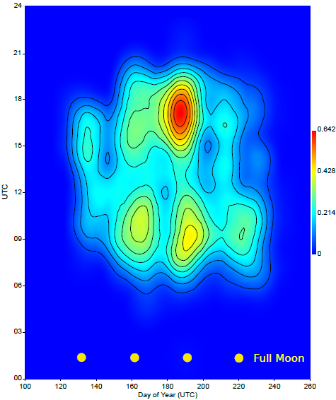
Figure 1 gives a concise depiction of the results. After considerable averaging solar and lunar tides clearly could be identified in Es forming. Whereas the solar tides are diurnal atmospheric oscillations caused by the local solar heating of the Earth the roughly monthly lunar tides are understood as a consequence of the gravitational pull of the Moon.
Fig. 1: Contour map of all received reports ordered by UTC and day, smoothed by a triangular kernel function. The report-density is colour coded. The recording period is May to August 2021. The dates of full moon are indicated.
If you want to read more you may take a look at the full study being published in the Journal of the International Meteor Organization: Kaufmann W. (2021) "Study of Sporadic E Occurrence in Europe 2021". WGN, The Journal of the IMO, 49:5, 114-119. You can read the article here.
However, the midlatitude Es forming is not only a diurnal phenomenon but also shows a perspicuous seasonal dependence that is marked by a pronounced summer maximum:
The role of meteoric influx and the geomagnetic disturbance on the seasonal forming of sporadic E over Europe
It is suggested that the seasonal sporadic E layer forming is determined by the supply of the atmosphere with metallic ions originating from incoming ablating meteoroids. However, this is controversly discussed in litrature. No clear picture can be gained about the influence of the meteoric influx on Es forming. Hence, the aim of this second study is to analyse the situation in Europe.
This time, the occurrence of Es was derived from daily Es layer critical frequency (fo Es) of 6 different European ionosondes. Thereby, the level of the frequency directly depends on the concentration of free electrons in the Es layer. A one year time series of the fo Es was considered. Forward scattered radio waves off ionised meteor trails were employed as an estimate of the influx of meteors over Europe. Additionally the daily geomagnetic Ap-Index was included in the analysis as a suspected influencing factor of Es-forming.
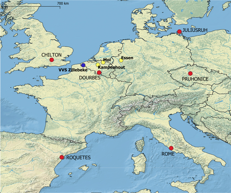
The analysis was performed for the time period 2020-01-01 to 2020-12-31. The radio observed number of daily meteors were provided by three receiving stations, located at Kampenhout, Mol and Essen. They employed the VVS-beacon at Zillebeke as transmitter at 49.99 MHz. From the European ionosondes Chilton, Juliusruh, Pruhonice, Dourbes, Roquetes and Rome data about Es layer critical frequency (fo Es) were retrieved from the Lowell GIRO Data Center (LGDC). The ionosondes were picked approximately on a circle around these meteor measuring stations or being directly adjacent, respectively, see Fig. 2. The planetary Ap-Indices were downloaded from the GFZ German Research Centre for Geosciences.
Fig. 2: Positions of the six Ionosondes (red), the three radio observation stations (yellow) and the applied transmitter (blue). Map made with Natural Earth.
Each ionosonde performed a couple of fo Es-measurements per day. For reducing them to a one day value the fo Es maximum value per day and ionosonde was taken. Thereby only those measurements were taken into account that had an auto-scaling confidence score ≥ 75. From the 8 daily 3h-Ap-Index measurements the maximum-value per day was taken. From the three radio meteor observing stations daily count rates (dCR) were derived. To each of these time series a 25-day moving average was applied. Hereby, short-term daily fluctuations were balanced out, long-term trends became visible. Subsequently the smoothed time series were normalised to 0-1. From the time series of the six ionosondes as well as of the three radio meteor observing stations a daily mean was calculated. Thus three basic measures were available: fo25 Es, Ap25 and dCR25. For further smoothing at least these three time series underwent a decomposition extracting the 10 day trend component: fo25 Es(trend), Ap25(trend) and dCR25(trend).
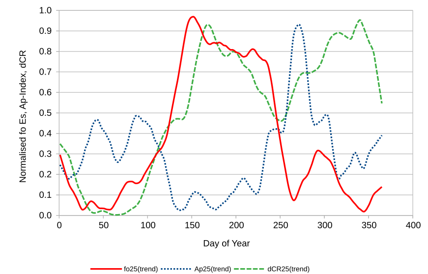
Fig. 3 shows the course of fo25 Es(trend), dCR25(trend) and Ap25(trend). Looking at the fo25 Es(trend) curve it should be pointed out, that an Es layer obviously was present throughout the year. However, its electron density only shows a pronounced summer maximum in May to August, a small local maximum in October and a second small local maximum in January. The dCR25(trend) curve shows two broad maxima: one in May to August and one in October to December. Also the Ap25(trend) has a seasonal shaped time course.
Fig. 3: The smoothed and normalised curve progression of critical frequency of the Es layer (fo25 Es(trend), red solid line), the meteor counts (dCR25(trend), dashed green line) and planetary A-Index (Ap25(trend), blue dotted line) in the year 2020.
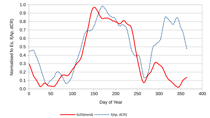
The occurrence of the summer maxima of both the fo25 Es(trend) and dCR25(trend) is astonishingly synchronous. The same is true for the minimum of Ap25(trend). Combining dCR25 and Ap25 could lead to an even better approximation to fo25Es. Therefore, a simple additive model was adopted:
f(Ap, dCR) = -Ap25(trend) + dCR25(trend)
The result is depicted in Fig. 4. In the time period from about February-September the f(Ap, dCR) curve correlates well with the fo25Es(trend) curve. The small local October maximum of fo25 Es(trend) initially follows the f(Ap, dCR) curve. However, with increasing temporal distance from the summer the degree of correlation decreases fast. Especially in November and December both curves show the largest deviation between them.
Fig. 4: The smoothed and normalised curve progression of critical frequency of the Es layer (fo25 Es(trend), red solid line) and combined meteor counts / Ap-Indices (f(Ap, dCR), blue dotted line) in the year 2020.
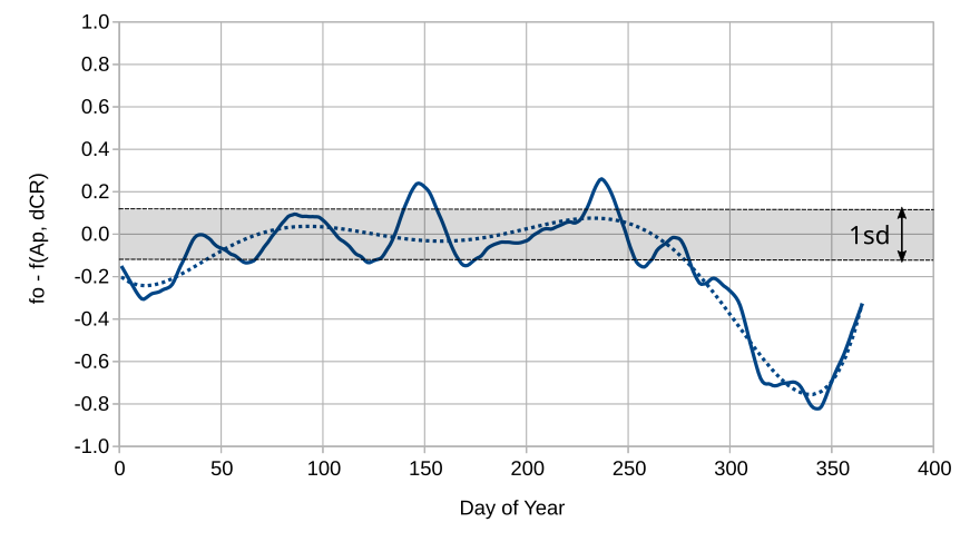
To evaluate their match in more detail the difference between the time series of fo25Es(trend) and f(Ap, dCR) was calculated and plotted in Fig. 5. The standard deviation (sd) of the calculated difference was used as matching-criterion. The range of one sd was centred around the zero line in Fig. 4. Thus the time periods could be estimated in which the difference between fo25Es(trend) and f(Ap, dCR) is within the span of one sd. Using this approach an essentially continuous match was found from February to September 2020 (days 32-273, corresponding to Feb. 1st and Sep. 29th, respectively).
Fig. 5: Plot of the difference between fo25Es and f(Ap, dCR) as shown in Fig. 4. The standard deviation centred around zero and a smoothing polynomial of 6th order (dotted line) are indicated.
This result does not support any of the conflicting data in the literature. On the one hand there is a remarkable match in the temporal evolvement of the combined meteor count rates / Ap-Indices and the Es layer critical frequency from February to September. On the other hand the same factor combination is not able to explain the low electron density of the Es layer from October to January. Following, it must be assumed that the seasonal variation of these two factors do not seem to play a key role in the seasonal variation of Es forming generally or at least during autumn-/winter. However, their surprising correlation with the Es occurrence during nine months of the year may assign them a modulating effect.
An explanation for the diverse findings could result from different methods used to estimate the meteoric influx. None of the used techniques (radar backscatter, forward scatter, visual) is capable to deliver a continuous 24 h observation based on a spatially uniform responsivity over the whole hemisphere. The distribution of detectable meteoroid masses also differs between the techniques and observing stations. This may strongly bias the estimate of meteoric influx.
Moreover, it should kept in mind, that seasonal different wind regimes in the MLT could be responsible for the seasonal variation of Es layer forming. Recently, a large number of neutral wind measurements from the Ionospheric Connection Explorer (ICON) mission (Immel et al., 2018) became available, providing an opportunity for direct comparison of Es with the local wind shear.
Acknowledgment
Meteor data kindly were provided by Felix Verbelen (personal communication) as well as Chris Steyaert and WHS Essen via RMOB. This paper uses data from the Juliusruh Ionosonde which is owned by the Leibniz Institute of Atmospheric Physics Kuehlungsborn, from the ionospheric observatory in Dourbes, owned and operated by the Royal Meteorological Institute (RMI) of Belgium, from the Observatory of Ebre, Spain, from the Chilton ionosonde operated by the Rutherford Appleton Laboratory, from the Průhonice Observatory of the Institute of Atmospheric Physics CAS and from the Rome Observatory of the Istituto Nazionale di Geofisica e Vulcanologia. The Ap-Index is taken from the GFZ German Research Centre for Geosciences.
Reference
This work also was published in the Journal of the International Meteor Organization: Kaufmann W. (2022) "The role of meteoric influx and the geomagnetic disturbance on the seasonal forming of sporadic E over Europe". WGN, The Journal of the IMO, 50:2, 62-65. You can read the article here.
